Demo
Use nldi_xstool function get_ext_bathy_xs to extend measured ADCP gage cross-section to on-land topography
As the current format of the bathymetry csv file is in flux, the function assumes the bathy file has lat lon positions and elevation. The user can specify the headings in the file, for example below, ‘Lon_NAD83’.
It is assumed that the bathy file positions are in EPSG:4326, but by specifying the EPSG code for the bathy data, it should handle different input projections.
Returned is a Geopandas Dataframe, using standard geopandas functions the dataframe can be reprojected and save to a file of users choice.
[1]:
%matplotlib inline
from pathlib import Path

import matplotlib.pyplot as plt
import py3dep
from shapely.geometry import LineString

from nldi_xstool.ancillary import get_ext_bathy_xs, query_dems_bbox

file = Path("../../data/09152500_2019-10-25_bathymetry.csv")
print(file.exists())
True
[2]:
xscomp = get_ext_bathy_xs(file, 50, "Lon_NAD83", "Lat_NAD83", "Bed_Elevation_meters_NAVD88", "epsg:4326")
xscomp
# code == 1 is original bathy, code == 0 is extended cross-section, station is distance from left bank.
# elevation values are in meters
[2]:
| spatial_ref | elevation | geometry | code | station | |
|---|---|---|---|---|---|
| 0 | epsg:4326 | 1417.116815 | POINT (-108.45195 38.98363) | 0 | 0.000000 |
| 1 | epsg:4326 | 1417.121930 | POINT (-108.45194 38.98363) | 0 | 0.999999 |
| 2 | epsg:4326 | 1417.125674 | POINT (-108.45193 38.98363) | 0 | 1.999999 |
| 3 | epsg:4326 | 1417.135304 | POINT (-108.45192 38.98362) | 0 | 2.999998 |
| 4 | epsg:4326 | 1417.139553 | POINT (-108.45191 38.98362) | 0 | 3.999997 |
| ... | ... | ... | ... | ... | ... |
| 145 | epsg:4326 | 1416.964678 | POINT (-108.45033 38.98331) | 0 | 143.599675 |
| 146 | epsg:4326 | 1417.221317 | POINT (-108.45032 38.98331) | 0 | 144.599676 |
| 147 | epsg:4326 | 1417.341967 | POINT (-108.45031 38.98331) | 0 | 145.599676 |
| 148 | epsg:4326 | 1417.402990 | POINT (-108.4503 38.9833) | 0 | 146.599677 |
| 149 | epsg:4326 | 1417.440459 | POINT (-108.45029 38.9833) | 0 | 147.599678 |
150 rows × 5 columns
[6]:
xstmp = xscomp.to_crs("epsg:3857")
p1x = xstmp.geometry[0].x
p1y = xstmp.geometry[0].y
p2x = xstmp.geometry[len(xstmp) - 1].x
p2y = xstmp.geometry[len(xstmp) - 1].y
xsline = LineString([(p1x, p1y), (p2x, p2y)])
xslineb = xsline.buffer(200)
bbox = xslineb.bounds

dem = py3dep.get_map("DEM", bbox, resolution=1, geo_crs="epsg:3857", crs="epsg:3857")
Note there is a function query_dems_bbox in the acillary package of nldi-xstools.
The method takes a bounding box in lon/lat (epsg:4326) coordinates and returns the available resolutions of 3DEP DEM topography. This can be used to provide context to the quality of topography the get_ext_bathy_xs function is using. The function always requests 1m resolution, which will simply return the best available resolution at 1m horizonal scale. Here there is 1m resolution available.
[7]:
bbox_latlon = tuple(xscomp.total_bounds.tolist())
query_dems_bbox(bbox_latlon)
[7]:
{'res_1m': True,
 'res_3m': False,
 'res_5m': False,
 'res_10m': True,
 'res_30m': True,
 'res_60m': False}
[8]:
def pltcolor(lst):
    cols = []
    for l in lst:
        if l == "0":
            cols.append("red")
        else:
            cols.append("blue")
    return cols


cols = pltcolor(xscomp.code.values)
[9]:
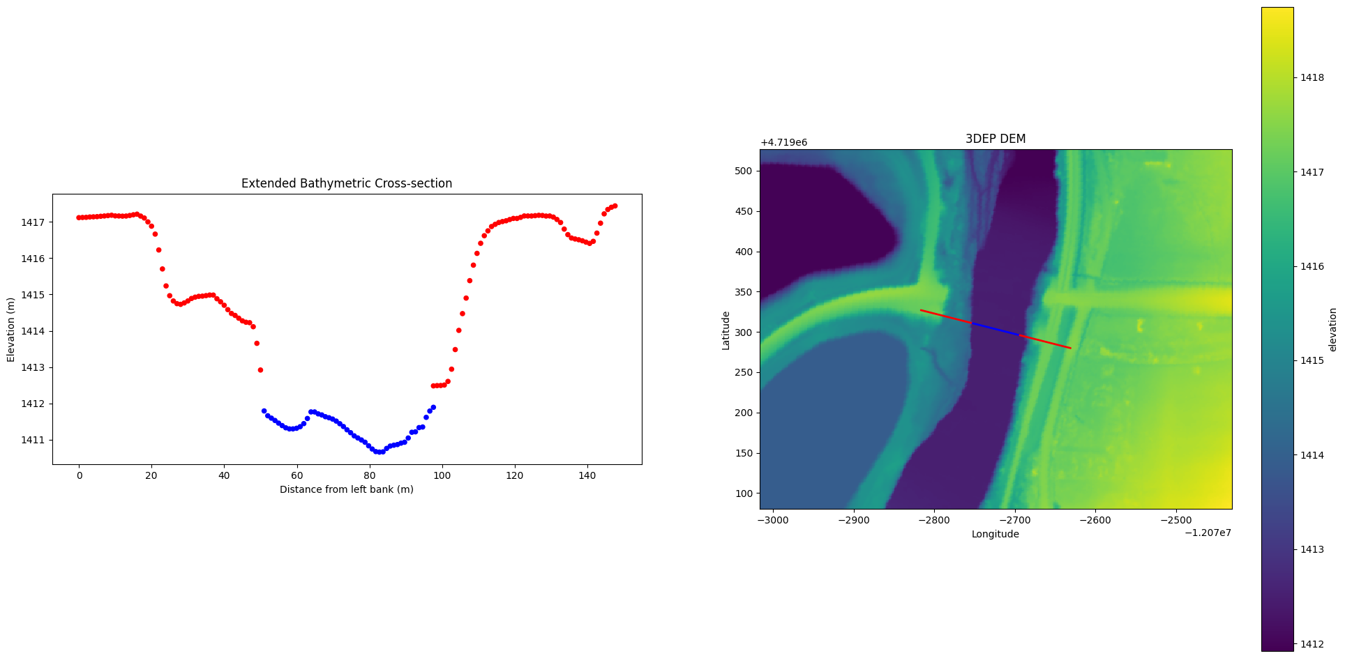
fig, ax = plt.subplots(1, 2, figsize=(24, 12))
ax[0].scatter(xscomp.station.values, xscomp.elevation.values, s=20, c=cols)
ax[0].set_xlabel("Distance from left bank (m)")
ax[0].set_ylabel("Elevation (m)")
ax[0].set_title("Extended Bathymetric Cross-section")
ax[0].set_aspect("10")

dem.plot(ax=ax[1])
ax[1].scatter(xstmp.geometry.x, xstmp.geometry.y, s=1, c=cols)
ax[1].set_aspect("equal")
ax[1].set_xlabel("Longitude")
ax[1].set_ylabel("Latitude")
ax[1].set_title("3DEP DEM")
[9]:
Text(0.5, 1.0, '3DEP DEM')
Notice the returned cross-section is a GeoPandas Dataframe and Geopandas functions can be used to save or reproject the file.
[10]:
print(type(xscomp))
<class 'geopandas.geodataframe.GeoDataFrame'>